BSSRDF

Duan gao

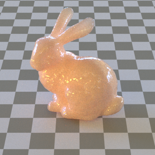
Bunny rendered by my own renderer Elegans.

BSSRDF aims to simulate volume scatterings using simplified assumption.

Separate BSSRDF

Split the BSSRDF into 3 parts: (Eq 11.7 in PRRT-v3)

About c (normalized factor),

$$\int_\Omega S_w(w_i) cos\theta d\omega_i = 1 \\ c = \int_{0}^{2\pi} \int_0^{\pi/2} {(1-F(cos\theta))} sin\theta cos\theta d\theta d\phi$$

And assume the $S_p$ is only related to $||p_o - p_i||$:

$$S_p(p_o, p_i) = S_r(||p_o - p_i||)$$

And the render equation:

Next I will introduce $S_r$ of normalized diffusion BSSRDF model and how to important sampling this BSSRDF.

Normalized diffusion BSSRDF

The key idea is using Exp function to approximate $S_r$ (including single-scattering and multiple-scattering).

• $S_r$ formula (using mean free path $l$ as parameter )

  From equation 3 in [1],

  • change $A$ to $\rho_{eff}$, because $A$ in dipole diffusion represents the internal reflection parameter;
  • $\rho_{eff}$ represents effective albedo, which is described in PBRT-v3 eq 11.11)

  $$S_r(r) = \rho_{eff} s \frac{e^{-sr/l} + e^ {-sr/(3l)}}{8\pi lr}$$

  where $r$ is the distance between $p_o$ and $p_i$, $s$ is scale factor and $l$ is mean free path length.

• Another formula (using diffuse mean free path $l_d$ as parameter)

  Compute $l_d$ and $s$ from physically based parameters ($\sigma_t$, $\sigma_a$, $g$, $\eta$):

  1. $l_d$ (diffuse mean free path)
  $$D = (\sigma_a + \sigma_a) / (3\sigma_t^2)\\ \sigma_{tr} = \sqrt{\sigma_a / D} \\ l_d = 1 / \sigma_{tr} \\$$

  2. $s$ (scale factor)

     $$\sigma_s' = \sigma_s * (1-g) \\ \sigma_t' = \sigma_s' + \sigma_a \\ \alpha' = \sigma_s' / \sigma_t'\\ \begin{align*} \rho_{eff} = & \int_{0}^{\infty} 2\pi rS_r(r) dr \\ = & \frac{\alpha'}{2} (1 + e^{-\frac{4}{3}A\sqrt{3(1-\alpha')}}) e^{-\sqrt{3(1 - \alpha')}} // [4] \end{align*}$$

$S_r$ (define $d = l_d/s$):

[1] Christensen P H. An approximate reflectance profile for efficient subsurface scattering[C]//ACM SIGGRAPH 2015 Talks. ACM, 2015: 25.

https://graphics.pixar.com/library/ApproxBSSRDF/paper.pdf

[2] Jensen H W, Marschner S R, Levoy M, et al. A practical model for subsurface light transport[C]//Proceedings of the 28th annual conference on Computer graphics and interactive techniques. ACM, 2001: 511-518.

https://http://graphics.stanford.edu/papers/bssrdf/bssrdf.pdf

Importance Sampling BSSRDF

There are two main approaches to implement BSSRDF model in physically based renderer.

• precompute irradiance in point cloud which sampled uniformly and compute the contribution in rendering.

  For example, the implementation in Mitsuba dipole.cpp.

• importance sampling the BSSRDF directly in rendering.

  More details about importance sampling the BSSRDF can be found in Section 6 of [1] and [2].

In the normalized diffusion BSSRDF model implementation, I use the second approach.

1. Sample BSSRDF and corresponding pdf

It is nontrivial to sample a neighborhood point of $p_o$ based on profile $S_r$.

1.1 Basic disk-based BSSRDF sampling

In the disk based sampling strategy, we map the 1D profile $S_r$ to 3D point in the surface geometry.

The key idea is :

• using $R_{max}$ to define a bounding sphere of $p_o$, the sampled $p_i$ will located in some position on this sphere.

  

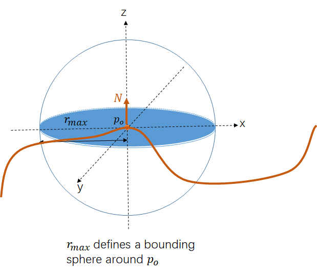
• sample $r$ from $S_r$ ($r\in (0,R_{max})$ [we need to map this radius value to a 3D point].

  

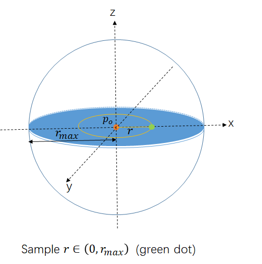
• sample angle $\phi$ ($\phi \in (0,2\pi)$) of the disk.

  

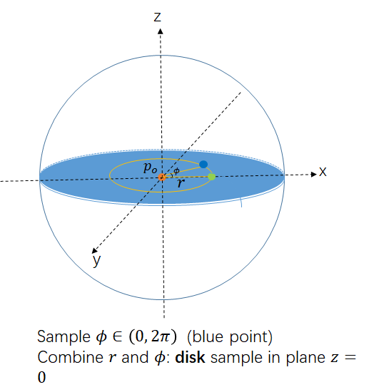
• project the point on 2D-disk to 3D sphere.

  

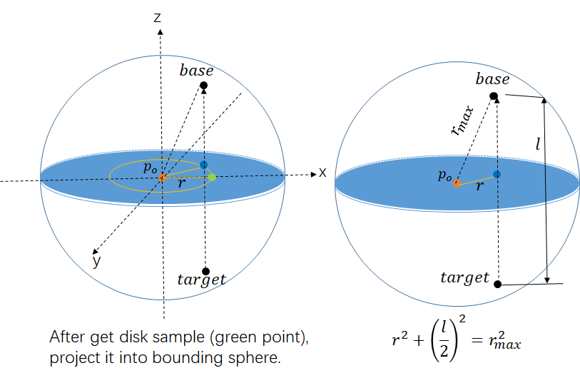
• emit probe ray (from base to target) and find the interaction which serve as the sampled point $p_i$.

  The contribution is:

  $$\frac{S_r(||p_o - p_i||)}{PDF_{disk}} \frac{1}{|z\cdot N_{p_i}|} \label{eq9}$$

  

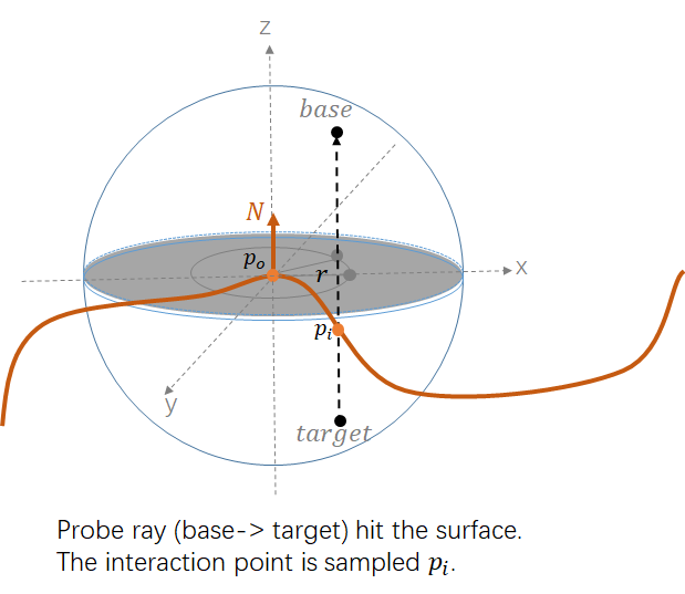
1.2 Axis and channels sampling

Using normal vector $N_{p_o}$ as the axis $z$ will lead to high variance in some sharp corners. (due to the dot product of $N_{p_i}$ and $N_{p_o}$ will be very small (close to zero)) :

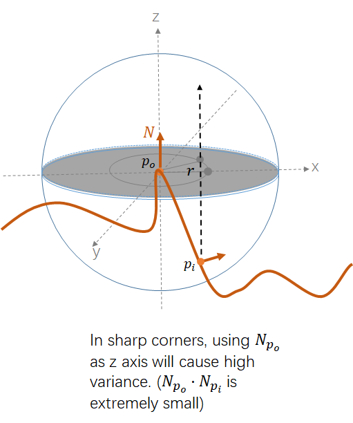
The solution is picking z axis from $[N_{p_o}, B_{p_o}, T_{p_o}]$ randomly .

For the channels, each channels may have different $S_r$ profiles, so we can also randomly pick one channel from R,G,B.

Now the contribution of each sample is ($Eq-\ref{eq9}$) :

For the axis and channel sampling, we use MIS to combine them (regarding each axis and channel as one sampling strategy):

Recall the MIS:

$$\sum_{i=1}^n \frac{1}{N_i}\frac{f(X_i) w_i(X_i)}{p_i(X_i)} \\ \sum_{i=1}^n \frac{f(X_i) w_i(X_i)}{p_i(X_i)} (if\ N_i=1\ for\ every\ strategies)$$

and $w_i(X_i) = \frac{p_i(X_i)}{\sum_jp_j(X_j)}$.

=>

$$\begin{align*} & \sum_{i=1}^n \frac{f(X_i) \frac{p_i(X_i)}{\sum_jp_j(X_j)}}{p_i(X_i)} \\ = & \sum_{i=1}^n \frac{f(X_i)}{\sum_jp_j(X_j)} \\ = & \frac{1}{\sum_jp_j(X_j)} \sum_{i=1}^n f(X_i) \end{align*}$$

1.3 Sampling scheme (NormalizedDiffusionBSSRDF::Sample)

• sample vertical axis randomly $[N_{p_o}, B_{p_o}, T_{p_o}]$

• sample channel randomly [r,g,b]

• sample $r_{max}$ from $S_r$ to get bounding sphere // [remain] how to sample from $S_r$

• sample $r \in (0, r_{max})$ from $S_r$ and angle $\phi$ in disk // [remain] how to sample from $S_r$

• project point in disk into bounding sphere to get base and target

• use probe ray (base => target) to find all possible interactions and random pick one (serve as $p_i$)

• evaluate the BSSRDF $S$

  $$S(p_o, \omega_o, p_i, \omega_i) = \frac{1}{\pi}(1-F(\omega_o)) S_p (p_o,p_i) S_\omega(\omega_i) \\ S_p(p_o, p_i) = S_r(||p_o - p_i ||) \\ S_r(r) = \rho_{eff} \frac{e^{-r/d} + e^{-r/(3d)}}{8\pi d r}\\$$

  In the implementation, $S_\omega(\omega_i)$, $\frac{1}{\pi}$, $1-F(\omega_o)$ are considered separately.

  For NormalizedDiffusionBSSRDF::Sample(), we only need to return $S_p$.

 

For $1-F(\omega_o) = F_t(\omega_o)$ , it is already considered in the BRDF (glass material). It is the pdf of transmit and only need to consider BSSRDF in this case.

 

For $\frac{S_\omega(\omega_i)}{\pi}$ , it is considered in $NormalizedDiffusionBSSRDF::Sw()$, which is called in NormalizedDiffusionAdaptor::Eval()

1.4 Pdf of above sampling (NormalizedDiffusionBSSRDF::Pdf_Sample)

For n sample strategies, the estimator is:

So the total pdf is $\sum_j {p_j(X_j)}$ (the pdf of all strategies).

For each $p_j(X_j)$, ( $Eq-\ref{eq10}$ )

$|z\cdot N_{p_i}|$ is trivial to evaluate, $PDF_{disk}$ will be introduced in next part.

2. Sample $S_r$ and $PDF_{disk}$

How to sample $r$ from $S_r$ profile?

Recall Monte Carlo estimator for $f(x)$ is $\frac{1}{N}\sum_i f(X_i)/ p(X_i)$,

And the PDF should satisfies:

$$\int p(x)dx = 1 \\ \forall x, p(x) \ge 0 \\$$

Inversion method to sample $X_i$ from $p(x)$:

1. compute CDF:$P(x) = \int^x_{-\infty} p(x) dx$
2. inverse of CDF: $P^{-1}(x)$
3. uniform random number $\xi\in(0,1)$
4. $X_i = P^{-1}(\xi)$

Recall $S_r$:

$S_r'$ satisfies: (integration in polar coordinates is always 1)

So the desired PDF is proportional to $S_r$.

Assume $PDF = c S_r$,

So the PDF is $cS_r = S'_r$

And the CDF is:

However, the CDF is not analytically invertible.

There are too methods to solve this problem.

1. We can use MIS to sample the 2 exp term separately:

   • Strategy 1(for first exp term)

     Assume the PDF is $c\ \frac{e^{-r/d}}{r}$

     $$\int_0^\infty \int_0^{2\pi} r ce^{-r/d}/r\ \mathrm{d}r \mathrm{d}\phi = 1 \\ \int_0^\infty 2\pi c e^{-r/d} = 1\\ e^{-r/d}(-d) 2\pi c|_0^\infty = d2\pi c = 1\\ c = \frac{1}{2\pi d}$$

     So the PDF is $\frac{e^{-r/d}}{2\pi d r}$

     CDF is:

     $$\int_0^r \int_0^{2\pi} r \frac{e^{-r/d}}{2\pi d r} drd\phi = \int_0^r \frac{e^{-r/d}}{d} dr = -e^{-r/d} |_0^r = -e^{-r/d} + 1$$

     $CDF^{-1}$ :

     $$\xi = -e^{-r/d} + 1\\ r = -d\log(1-\xi)$$

   • Strategy 2 (for second exp term)

     Assume the PDF is $c e^{-r/(3d)}/r$

     $$\int_0^\infty \int_0^{2\pi} r ce^{-r/(3d)}/r\ \mathrm{d}r \mathrm{d}\phi = 1 \\ \int_0^\infty 2\pi c e^{-r/(3d)} = 1\\ e^{-r/(3d)}(-3d) 2\pi c|_0^\infty = 3d2\pi c = 1\\ c = \frac{1}{6\pi d}$$

     So the PDF is $\frac{e^{-r/(3d)}}{6\pi d r}$

     CDF is:

     $$\int_0^r \int_0^{2\pi} r \frac{e^{-r/(3d)}}{6\pi d r} drd\phi = \int_0^r \frac{e^{-r/(3d)}}{3d} dr = -e^{-r/(3d)} |_0^r = -e^{-r/(3d)} + 1$$

     $CDF^{-1}$:

     $$\xi = -e^{-r/(3d)} + 1\\ r = -3d\log(1-\xi)$$

2. Precompute the $CDF^{-1}(r)$ when $d=1$ , and multiply d in rendering.

   $$CDF = 1 - \frac{1}{4}e^{-r/d} - \frac{3}{4}e^{-r/(3d)} \\ \stackrel{d=1}{==} 1-\frac{1}{4}e^{-r} - \frac{3}{4}e^{-r/3}$$

   $CDF^{-1}$ : $\xi => r$

     # python script to precompute the inverse CDF
       
     import scipy
     from math import exp
     
     def F(r, xi):
         return 1.0 - 0.25 * exp(-r) - 0.75 * exp(-r/3) - xi
     
     steps = 1024
     x0 = 0
     R = []
     XI= []
     for i in range(steps + 1):
         xi = 1.0 / (steps) * r
         r = scipy.optimize.newton(F,x0,args=(xi,))
         x0 = r
         XI.append(xi)
         R.append(r)
     
    print(R)
   

   Sample $S_r$: (precompute $CDF^{-1}$)

   given random variable $\xi \in (0,1)$:

   • locate $\xi$ in $CDF^{-1}$ array.
   • Linear interpolate two neighborhood.
   • multiply d.

   Pdf: just return $S_r'$.

[1] Christensen P H. An approximate reflectance profile for efficient subsurface scattering[C]//ACM SIGGRAPH 2015 Talks. ACM, 2015: 25.

https://graphics.pixar.com/library/ApproxBSSRDF/paper.pdf

[2]King A, Kulla C, Conty A, et al. BSSRDF importance sampling[C]//ACM SIGGRAPH 2013 Talks. ACM, 2013: 48.

http://www.aconty.com/pdf/bssrdf.pdf

[3] http://shihchinw.github.io/2015/10/bssrdf-importance-sampling-of-normalized-diffusion.html

Combining BSSRDF in path tracing

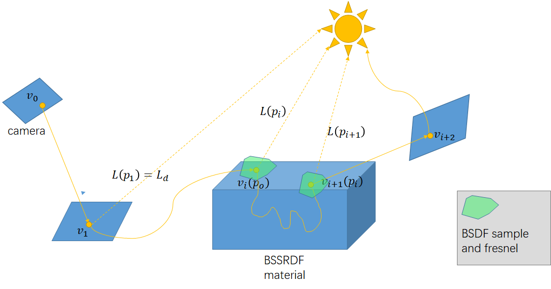
• direct lighting of BSSRDF compute in $p_i$.

• indirect lighting (from $p_i$ sample the next direction)

• In $p_o$ and $p_i$, there are BSDF sample happened (contains Fresnel transmit $F_t(\omega_i)$ and $F_t(\omega_o)$).

  (there are some discussions about the implementation details in [1])

[1] https://github.com/mmp/pbrt-v3/issues/19